War on Orange: Statistics

Are oranges getting better? Worse? How do we tell?

The oranges are very tricky and don't like to be measured. They are intermittent! They like to avoid detection and will shy away from getting your hand on them. The data is noisy: between one push and the next there is no necessary correlation between either the number nor the identity of the oranges being observed.

Fortunately, we have in our arsenal mathematical tools that may be used to coerce truth from the wily oranges.

Types of Transforms

Given a time-series of data...

• filters: transform the series of data giving back the same number of points (as defined for this purpose)

• reductions: give back a scalar value, such as a mean, median, or standard deviation

• windows: take a subset of the window for further analysis

Note that a hg push series is a time series

We should move towards an architecture where an arbitrary set of filters may be applied. So you could e.g. filter, filter, window, reduce.

Filters

• smoothing

Smoothing

Gaussian smoothing:

Gaussian smoothing applies a bell-shaped filter to data in order to remove high-frequency noise.

While the entirety of the bell curve may be used, it is more common to use a lower order form. The lowest order for is a 1-2-1 filter. In python, this looks like:

def smoothing_pass(data):
  if len(data) < 2:
    return data
  retval = [0 for i in data]
  for i in range(data):
    denom = 0.
    if i < len(data) - 1:
      retval[i] += data[i] + data[i+1]
      denom += 2.
    if i > 0:
      retval[i] += data[i] + data[i-1]
      denom += 2.
    retval[i] /= denom
  return retval

This function performs one pass of a smoothing filter, which for an interior node gives the average of two parts the value plus one part the value of each of its neighbors. Multiple passes of the smoothing function may be applied to the data to achieve even smoother results. The exact number of passes to use depends on the data to be smoothed -- too few passes and the data will be too rough, too many passes and the data will lose its shape. It should be noted that smoothing is a lossy operation.

For each pass of the above function, data propagates one node to the right and one node to the left. Often, it is desirable that smoothing take place over a wider swath of data but without the comparatively high coefficients given to the neighboring nodes. In this case, weighted smoothing may be used:

def smoothing_pass(data, weight=1.):
  if len(data) < 2:
    return data
  retval = [0 for i in data]
  for i in range(len(data)):
    denom = 0.
    if i < len(data) - 1:
      retval[i] += data[i] + weight*data[i+1]
      denom += 1. + weight
    if i > 0:
      retval[i] += data[i] + weight*data[i-1]
      denom += 1. + weight
    retval[i] /= denom
  return retval

A weight less than 1 is typically chosen. The lower the weight, the less smooth a single pass will be, so typically more passes are run for lower weights which allows information (data) to propagate from further away nodes. The average is still heavily weighted towards local nodes, but less dramatically so.

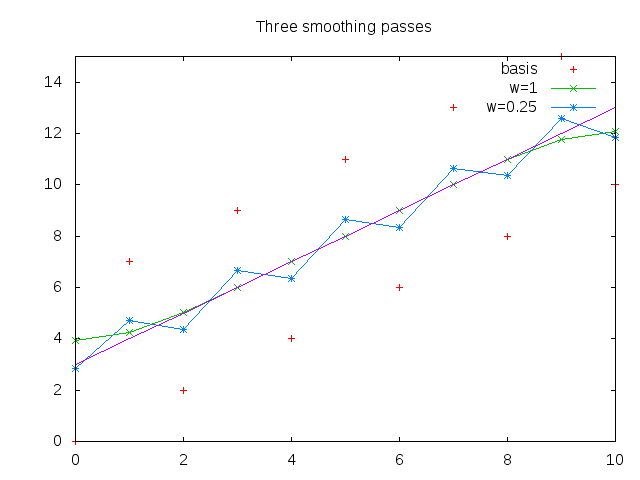
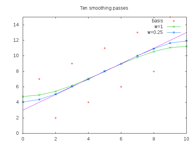
To illustrate how these filters behave, first apply them to a line that rises linearly from 3 to 13 but has -/+ 3 variation for odd/even numbers, respectively. Assuming that this is "noise" (it is high frequency), then smoothing should approximate a linear rise. A weight of 0.25 was used for the weighted smoothing and three and ten smoothing passes were ran.

It can be seen that unweighted (w=1) smoothing converged rapidly even with three iterations. With ten smoothing passes, the results are mostly the same, though the weighted (w=0.25) smoothing has better results along the edges. The endpoints are hard to get accurate with this type of filter as you only have information coming from one direction. Note that the results towards the endpoints are worse for ten passes at w=1 than at three passes. The results are over-smooth and would get even worse with more passes, eventually trending to a constant. This illustrates that the choice of number of passes and weight appropriate to given data is a function of the data. This may be automatically controlled if desired.

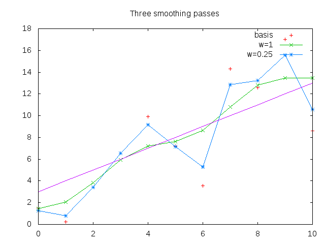
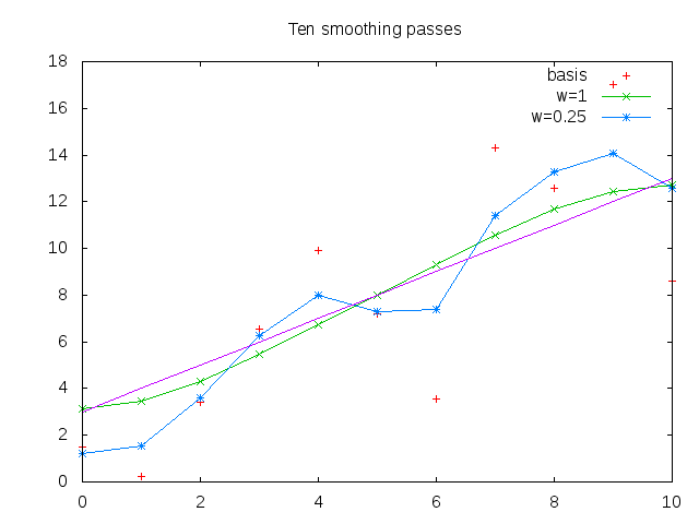
To give an example more illustrative of real noise, we take the same basis curve (linear rise from 3-13) and for each point add a random value from -6 to 6 to it. A high amount of noise was chosen both to be illustrative and because oranges are also very noisy. Note the small number of data points (11) hurts us in identifying the trend but is good for illustration.

Note that while these filters were applied iteratively, an equivalent coefficient matrix could have alternately been constructed and multiplied by the data vector for a given weight and number of iterations.

Low pass filters: TODO

Interesting Statistics

What are we really measuring? What does it mean? In order to combat the oranges, we must understand them. This means having in our arsenal creative measured quantities that tell a story.

Statistics should be identified that accurately and effectively convey trends in the data:

• oranges/push as a function of time (orange factor)
• most common failures as a function of time (topfails)
• for a given window, breakdown of oranges by bug number
  • in other words, are there a lot of different orange bugs?
  • is any of them a big chunk?
  • or are they highly scattered?
• push rate (number of pushes as a function of time; pushes/week, etc)
• occurance rate of orange bugs (per push) as a function of time

It is to be noted that these statistics are abstractions useful to tell a story. Fundamentally, there are discrete push events. These push events yield a certain set of oranges which are then starred.

Most Common Failures (topfails)

What particular orange bugs are most commonly seen? If I look at the last week of data, how would the oranges break down? Given the number of pushes, say, in the last week, how would these break down? Would there be a few orange bugs that, if eliminated, would significantly change the orange factor? Or are the oranges so scattered that it is unlikely that fixing any given orange would change the picture much? How does this differ from last week?